Highlights all the blanks in a list of data in Excel!

All Excel spreadsheets which are used for data analysis, calculation or manipulation; have large amounts of data and so it is very difficult to locate all the blank spaces within those Excel spreadsheet. The blank spaces in Excel spreadsheet could cause numerous issues including errors and breaks in formatting. This tutorial presents the easiest and simple ways to locate and highlight all blanks within the data.

---

Get yourself ready!

---

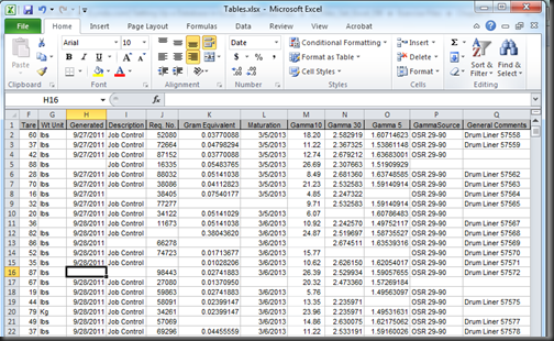
In the following example, we have an Excel sheet where several bank spaces are present there. We would use a automated method of Excel to search all the blank spaces and mark those cells with a different color says light blue.

---

Steps to highlights all the blanks in a list of data in Excel!

---

Step 1: Open the spreadsheet in Excel that you need to highlight the blank spaces.

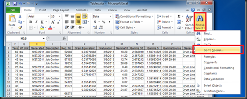
Step 2: From the opened file, click on Home tab. Under the Home tab, there is an option Find & Select and just click on that option Find & Select and then choose Go To Special and click on that option. This will brings the Go to Special dialog box.



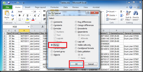
Step 3: From Go To Special dialog box, select the option Blanks and click  on OK.



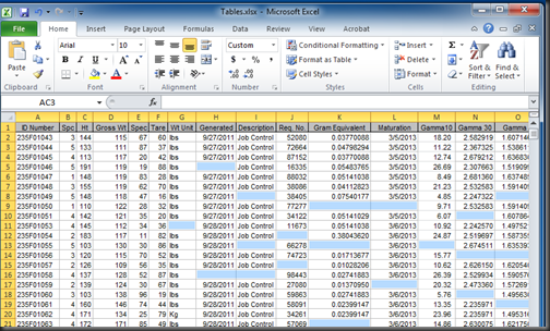
Step 4: Now, you will see that all of the blanks within the data spreadsheet have been highlighted.



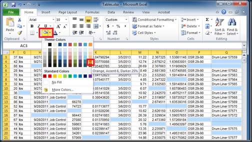
Step 5: Now, we would like to apply a format to all those blank cells. For example, we would like to fill all the blank cells orange color. So, we choose the color.  This now provides a contrasting visual indicator to locate blanks on the screen or when printed and anybody could easily figure out all the blank cells in the spreadsheet.



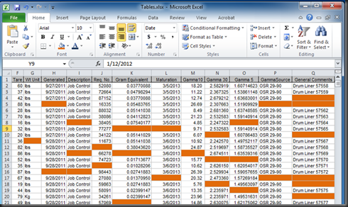
After applying the cell format, you will see that all the blank spaces are marked with orange color.

---

How this method works?

---

The Go To Special is a built-in find feature of Excel and provides several criteria to find data within the spreadsheet. When the Blanks are selected from Go To Special dialog box,  Excel quickly parsed through the data and select all those cells that contained no data i.e. the blank spaces. After that, with all of the blank cells selected, you would  easily apply a visual indicator in your spreadsheet.

---

Think more!

---

We use just the orange color as the indicator of the blank cells. However, it is possible to use other type of indicators like lines, characters, and so on.

Remove all formulas from a list of numbers using Excel

When we work any Excel sheets, data are existed on those sheets. These data can be come from other source or may be calculated from using equations or other ways. So, what to do to remove all the formulas. To remove the formulas, we click on within each cell that contains a formula and retype the answer hence removing the formula. To continue removing in this way may become tedious. But there is another alternate way. Following this tutorial, you will learn how to quickly remove all formulas from a row of data retaining the calculated answers.

---

Get yourself ready!

---

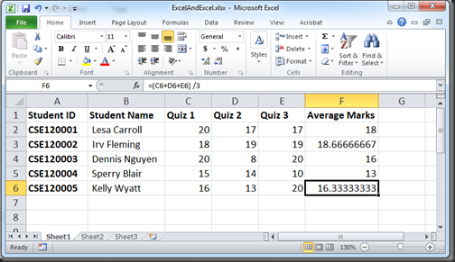
In the following example, we have an Excel sheet where in column F there are average quiz marks of some student. The quiz marks are calculated using formula. Our goal is to clear the formula from column F while retaining the value data:

---

Steps to remove all formulas from a list of numbers using Excel

---

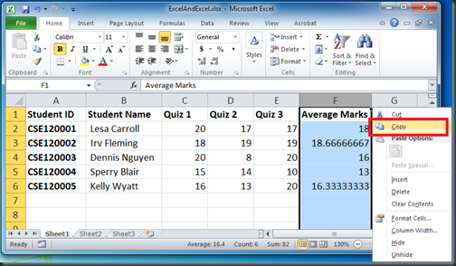
Step 1: Highlight i.e. select the the row or column or data that contains the formulas. After selecting, copy the information / data by choosing the Copy option.



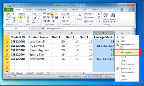
Step 2: Now, with the copied data, just right-click on column and choose Paste Special.



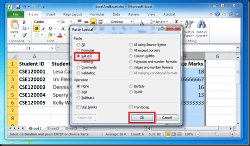
Step 3: After completing the above steps, you will see the Paste Special dialog box will be opened. Form the Paste Special dialog box, select Values and click on OK button.

---

How this method works?

---

The default copy and paste option of Excel, generally copy the text, the formulas, and the formatting. But when the paste special option is selected, it only paste the values  from the formulas when we choose Values from Paste Special dialog box

---

Think more!

---

Several functions including Paste Special have shortcut buttons in the Excel Ribbon which offer some quicker access. You can also do that from there.

How to start Excel

The basic tasks of Excel are for building a spreadsheet and then manipulating the data on the spreadsheet. Before performing any task we must have to start Excel. Starting Excel brings the Excel window onto the desktop and then we can use the program.

Note: In this tutorial, we discuss how to start Microsoft Excel 2010 program. This tutorial also more or less same for other version of Excel.

---

Steps to start Excel:

---

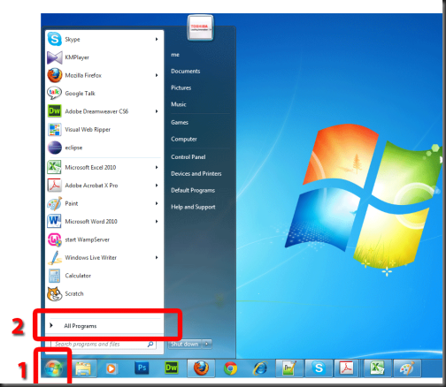
Step 1: Click on the "Start" menu of your computer. This brings the Start menu

Step 2: Click "All Programs" and the App Programs menu will be appeared



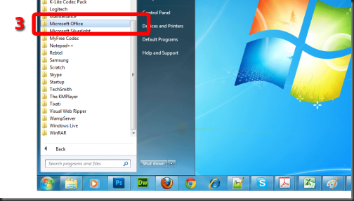
Step 3: Click “Microsoft Office” and Microsoft Office menu will be appeared



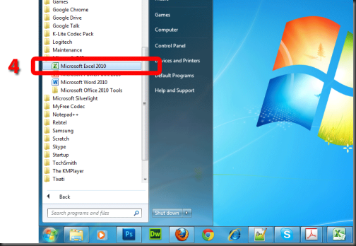
Step 4: Click “Microsoft Excel 2010”



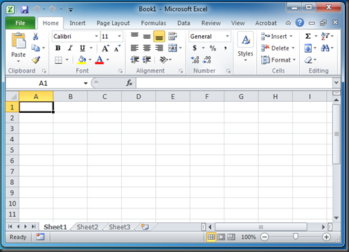
Completing the above steps, the Microsoft Excel window will be appeared on the desktop.



Note: When you have finished working with Excel, you could easily close the program by clicking the File tab and then clicking Exit.

Setting up an Excel spreadsheet

For any type of financial data, first we need to create an Excel spreadsheet to display or analyze data. Setting up an Excel spreadsheet is not difficult. In this tutorial, we would learn how to set up an Excel spreadsheet easily.

---

Reasons to set up an Excel spreadsheet

---

If the Excel is properly formatted, we could easily utilize many new layouts, formulas, and search functions throughout the spreadsheet for different purposes. Otherwise, it's not possible to do. That's why, the specific setup of spreadsheet is always extremely important.

---

Steps to set up an Excel spreadsheet

---

Before setting up an Excel worksheet, we must have to figure out label, identifier, and
value for proper formatting of the Excel worksheet and then we have to put all of them to the worksheet. Labeled data is placed as column headers, identifier information is placed within the fist column beneath its corresponding label and finally the values are then listed according to the label and identifier. [Note: For details about label, identifier and value, please read Common concepts to format any spreadsheet data].

For this tutorial, we use the following table as an example. In this table, there are some students quiz numbers with there names.

Step 1: Formatting Labels

Open a new Excel document and define all the labels. In this tutorial, Student ID, Student Name, Quiz 1, Quiz 2 and Quiz 3 are the labels. All these labels will allow us to know what information is being presented. So, we put the labels like the Excel spreadsheet.

Step 2: Formatting Identifier

After label mapping is completed, now need to define the Identifier. Identifiers are unique pieces of information which allows quick identification of value. In this example, the student ID would be the optimal identifier, as there may be two individuals with the same name.

Step 3: Formatting Values

We already completed the labels and identifiers for our financial data. Now, we need to add the values for those identifiers according to the labels and these values are the child data to the identifying student ID parent. Since the parent is student ID, the child values will be the individual student's names, and their quizzes marks.

And that’s all. Thus for any financial data at first we have to create a layout like the above for several reporting, graphing and summarizing data. Without the concept of Labels, Identifiers and Values, it is not possible to do any analysis type of work or graph related wok.

---

Tips and tricks

---

At the time of formatting data into an Excel spreadsheet, always try to split your data into the smallest piece possible.

Why Excel is used?

The popular Electronic Spreadsheet Program "Excel", could be be very useful for calculating financial, statistical and engineering information. Excel is used from individual households to Fortune 500 companies. Some of the usage of Excel are:

• Excel is very handy for performing calculations as lots of built-in formulas (simple and complex formulas) are included for basic math, statistics and even engineering functions.
• Creation of charts and graphs (like pie charts, bar graphs, 3-D graphs and even scatter-grams) are really simple using Excel.
• For complex work sometimes, one sheet result may need to use to other spreadsheet and this could be done using spreadsheet linking which helps to retyping or recopying the cell data to other spreadsheets.
• For visual representation of data, Excel provides lots of formatting option which makes the data more visually represented and meaningful.
• Excel not only deals with data but also make the data secure from unwanted changing or password protected from others.
• Excel provides different format data exporting features which could be used to import into Access, MySQL, MSSQL, Oracle etc.